Contents
Analysis: 20250611
!pip install nucleus-cdk | tail -n2from cdk.analysis.cytosol import platereader as pr
import matplotlib.pyplot as plt
import seaborn as sns
import warnings
# Filter warnings
warnings.filterwarnings('ignore')
# Initialize plotting
pr.plot_setup()Load the data
Provide a CSV file containing the data, and a platemap. This function returns both the data with the plate map mapped to it, and the platemap by itself, which is useful for certain tasks.
data, platemap = pr.load_platereader_data("./data/20250611-cytation3-pure-timecourse-gfp-ppk-mg-sweep-biotek-cdk.txt", "20250611-Mg-sweep-platemap.csv")Basic Plots
Kinetics
Kinetic time traces of every well on the plate
pr.plot_plate(data)<seaborn.axisgrid.FacetGrid at 0x791f190fd430>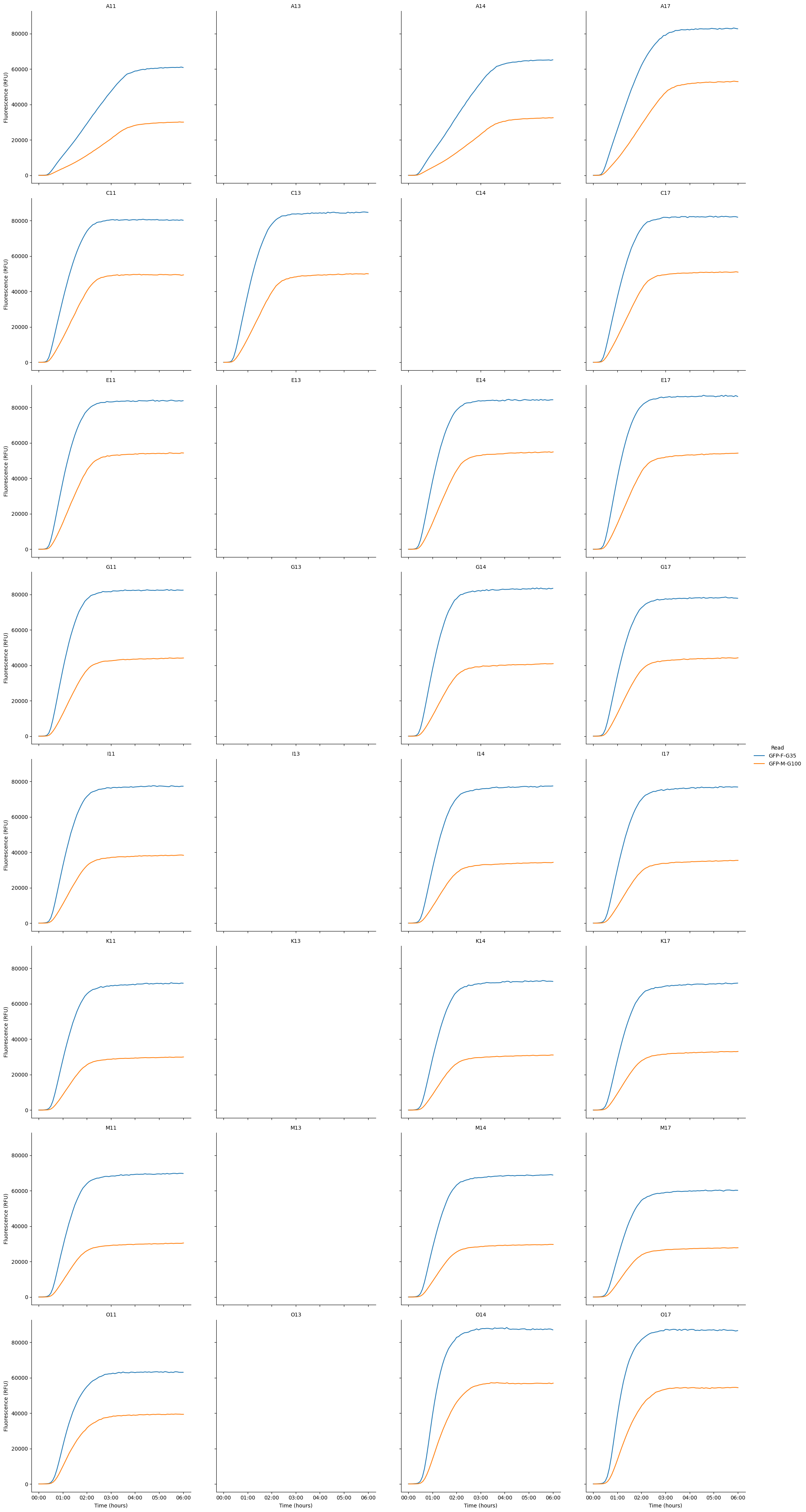
pr.plot_curves(data[data["Read"]=="GFP-F-G35"], units="Well", estimator=None, height=12)<seaborn.axisgrid.FacetGrid at 0x791f14515670>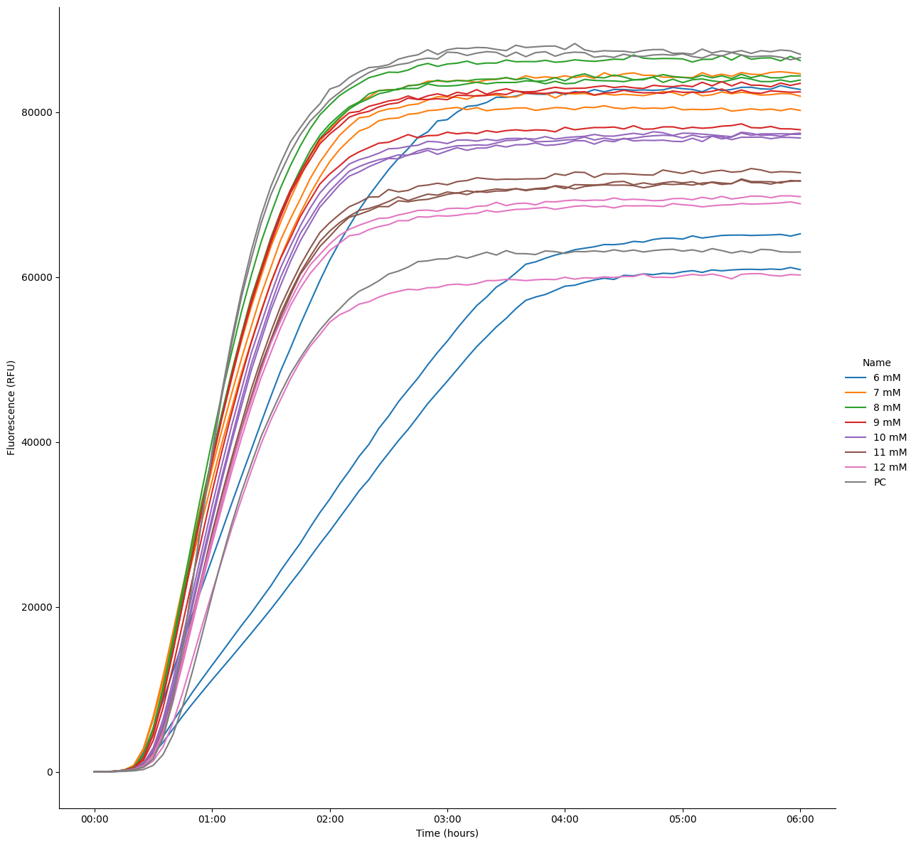
Steady state
Bar graph of steady-state endpoint of each sample. Steady state is calculated as the maximum fluorescence value over a 3-sample rolling average on the data.
steadystate = data.merge(pr.find_steady_state(data[data["Read"]=="GFP-F-G35"]).reset_index(), on="Well", how="left")
steadystate.loc[steadystate["Column"]==13, "Column"] = 14
sns.barplot(data=steadystate, x="Name", y="Data_steadystate", hue="Column")
<Axes: xlabel='Name', ylabel='Data_steadystate'>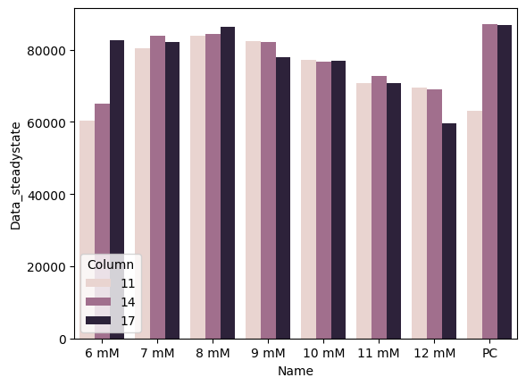
s= pr.plot_steadystate(data[data["Read"]=="GFP-F-G35"])
plt.xlabel("[Mg++]")
s.savefig("plot3")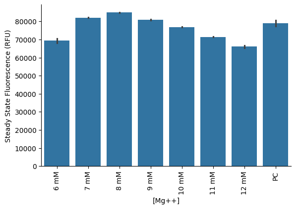
Kinetics Analysis
These functions calculate key kinetic parameters of the time series.
pr.plot_kinetics(data[data["Read"] == "GFP-F-G35"])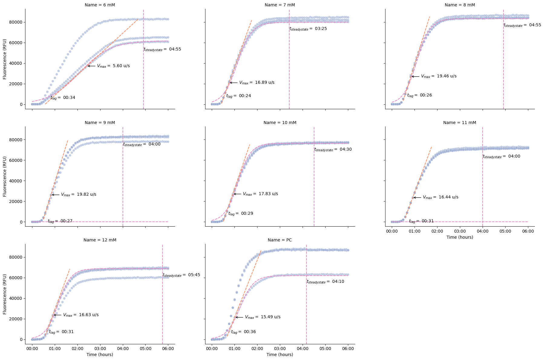
We can also calculate the kinetics and display the parameters as a table.
pr.kinetic_analysis(data) Velocity \
Time Data Max
Well Name Read
B1 pT7-deGFP 100 485/20,528/20 0 days 00:05:00 6.00 0.02
B2 pT7-deGFP 50 485/20,528/20 0 days 00:15:00 28.00 0.04
B3 pT7-deGFP 20 485/20,528/20 0 days 00:05:00 6.00 0.02
B4 pT7-deGFP 10 485/20,528/20 0 days 00:35:00 220.00 0.17
B5 pT7-deGFP 5 485/20,528/20 0 days 00:05:00 6.00 0.02
B6 pT7-deGFP 2 485/20,528/20 0 days 00:15:00 19.00 0.03
B7 pT7-deGFP 1 485/20,528/20 0 days 00:05:00 5.00 0.01
B8 pT7-deGFP 0 485/20,528/20 0 days 00:50:00 156.00 0.08
Lag \
Time Data
Well Name Read
B1 pT7-deGFP 100 485/20,528/20 -1 days +23:59:00 0.00
B2 pT7-deGFP 50 485/20,528/20 0 days 00:04:13.846153846 0.00
B3 pT7-deGFP 20 485/20,528/20 -1 days +23:59:00 0.00
B4 pT7-deGFP 10 485/20,528/20 0 days 00:13:25.882352941 0.00
B5 pT7-deGFP 5 485/20,528/20 -1 days +23:59:00 0.00
B6 pT7-deGFP 2 485/20,528/20 0 days 00:04:26.666666667 13.38
B7 pT7-deGFP 1 485/20,528/20 -1 days +23:58:45 0.00
B8 pT7-deGFP 0 485/20,528/20 0 days 00:16:05.217391304 0.00
Steady State Fit
Time Data L k x0
Well Name Read
B1 pT7-deGFP 100 485/20,528/20 0 days 00:25:00 6.00 0.00 0.00 0.00
B2 pT7-deGFP 50 485/20,528/20 0 days 02:40:00 132.00 0.00 0.00 0.00
B3 pT7-deGFP 20 485/20,528/20 0 days 00:20:00 6.00 0.00 0.00 0.00
B4 pT7-deGFP 10 485/20,528/20 0 days 02:45:00 679.00 0.00 0.00 0.00
B5 pT7-deGFP 5 485/20,528/20 0 days 00:20:00 6.00 0.00 0.00 0.00
B6 pT7-deGFP 2 485/20,528/20 0 days 02:35:00 108.00 106.53 0.00 2482.26
B7 pT7-deGFP 1 485/20,528/20 0 days 00:20:00 5.00 0.00 0.00 0.00
B8 pT7-deGFP 0 485/20,528/20 0 days 02:30:00 310.00 0.00 0.00 0.00